Previous lesson: Continuous bivariate data
R Intro to stats: Analysis of variance (ANOVA)
Analysis of variance (ANOVA) is a statistical test based on the general linear model that can extend the simple t-test of means. ANOVA can assess differences among more that two levels of a factor. It can also the effect of two factors simultaneously.
Learning objectives At the end of this lesson, the learner will be able to:
- describe how variance among and within groups (levels) is used in ANOVA to assess whether differences are significant.
- list three assumptions of ANOVA
- list conditions under which an ANOVA is robust to violations of its assumptions.
- perform Bartlett’s test to determine whether the residuals in an ANOVA are normally distributed.
- state the preferred test for determining whether variance among groups is heterogeneous.
- describe the relationship between a t-test of means and a single-factor ANOVA with two levels.
- explain why the cutoff level of P for significance must be adjusted for post-hoc pairwise comparisons.
- perform a Tukey honestly significant difference (HSD) test for pairwise comparisons.
- perform a Kruskal-Wallis non-parametric alternative to a single-factor ANOVA.
- (optional) use the
aov()function to set up a two-factor fixed effect ANOVA. - (optional) use a summary of the two-factor model to generate an ANOVA table.
- (optional) interpret a two-factor ANOVA table.
- (optional) describe an interaction term and explain how its significance affects the interpretation of the fixed effects.
- (optional) define random effect and describe its role in ANOVA.
- (optional) describe the role of a block in the design of an experiment.
- (optional) use the
lmer()function to set up a mixed linear model. - (optinoal) explain how including a random effect affects the power of ANOVA to detect the affect of a fixed effect.
- (optional) interpret the results of a mixed model ANOVA.
- (optional) describe the relationship between a paired t-test and a two-factor mixed model ANOVA.
Total video time: 62 m 31 s
Links
One-factor Analysis of Variance (ANOVA)
Introduction to ANOVA (2m13s)
How an ANOVA works (7m51s)
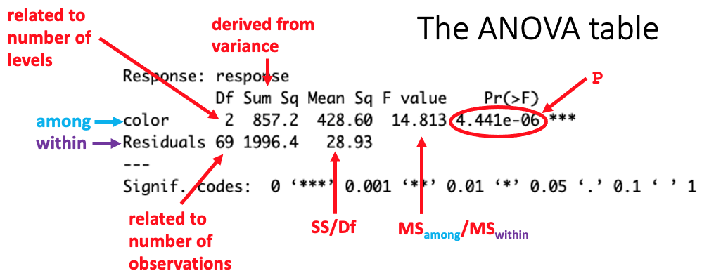
The within group variance is the variance of the residuals.
See this page for a diagram illustrating among and within group variation.
ANOVA format and assumptions (2m38s)
The commands to carry out a single-factor ANOVA are:
model <- lm(Y ~ X, data = data_frame)
anova(model)
The data = argument can be omitted if vectors or explicitly specified columns are used.
See this reference for more details about the robustness of ANOVA to violations of the homogeneous variance assumption.
Testing assumptions of ANOVA (5m07s)
Inputting the model as an argument of the plot() function generates plots showing the distribution of residuals and a normal quantile (Q-Q) plot of the residuals as was the case for linear regression. The residuals are grouped on the X axis by the predicted group means for Y.
The Shaprio-Wilkes test (used previously in other contexts) can be applied in ANOVA to test whether the residuals are normally distributed:
resid <- residuals(model)
shapiro.test(resid)
Bartlett’s test is often considered an overly conservative test for heterogeneity of variance. Levene’s test is the generally preferred alternative.
The car package provides access to the leveneTest() function:
leveneTest(log ~ color, data=ergDframe, center = mean)
Dropping the center = argument performs the Brown-Forsythe test (a variant that uses medians instead of means) instead of Levene’s test. See this page for information about the situations where the Brown-Forsythe test might be preferred to Levene’s test.
Analyzing the transformed data (3m55s)
ANOVA vs. t-test of means (2m44s)
A t-test of means and a single factor ANOVA with two levels produces an identical value of P. The calculated value of F in the ANOVA will be the same as the square of the calculated value of t in the t-test of means.
Post-hoc pairwise comparisons (4m03s)
To use the Tukey honestly significant difference (HSD) or Tukey-Kramer tests for post-hoc pairwise comparisons, you must first create an ANOVA object and pass it into the function:
anova_object <- aov(model)
TukeyHSD(anova_object)
For more details, see this page.
Kruskal-Wallis non-parametric alternative (2m31s)
To perform the non-parametric Kruskal-Wallis alternative to single-factor ANOVA, use:
kruskal.test(Y ~ X, data=data_frame)
Two-factor ANOVA with two fixed effects and interaction
Note: this is an optional advanced topic.
Two-factor ANOVA is also known as two-way ANOVA
References:
Some examples of setting up two-factor ANOVAs with some nice ggplot visualizations
Introduction to two-factor fixed effects ANOVA (2m04s)
Two-factor ANOVAs are somewhat controversial, particularly when they are used for hypothesis testing (to assess P). However, well designed, relatively large experiments with balanced design (equal sample size per group) may be safely analyzed using two-way ANOVA.
Fixed effects are factors that are controlled by the experimenter (vs. random effects). Randomized controlled trials (RCTs) have one or more fixed effects as their primary variable of interest.
Full factorial experimental design setup (3m16s)
A full factorial experiment has every combination of all levels of all factors.
In a balanced design, every combination of level has the same number of observations.
Setting up the model (5m04s)
The main effects of a model are the individual factors in the experiment. The interaction term is the combination of the main effects – a measurent of how main effects influence each other.
There are several ways to set up a two-factor ANOVA. To set up a full factorial model using the aov() function to generate an ANOVA object:
anova_object <- aov(Y ~ X1 + X2 + X1:X2)
where X1:X2 is the interaction term. A full factorial model includes every possible interaction term involving the main effects. A shortcut way to set up a full factorial model uses * instead of +:
anova_object <- aov(Y ~ X1 * X2)
Two-factor ANOVA table (1m37s)
Each row of a two-factor ANOVA table summarizes the statistics for one of the factors/effects in the design (main effects + interaction term).
First examine the interaction term. If it is significant, then the interpretation is over – the main effects will not have a clear interpretation. If the interaction term is not significant, the P values of the main effects may be examined to determine whether they have significant effects.
Running the two-factor ANOVA (3m24s)
Testing for normality of residuals and homogeneity of variance among groups are carried out in the same way as with a single-factor ANOVA. The Levene’s test function leveneTest() from the car package can only be used to test for homogeneity of variance when the model is full factorial (includes all interactions).
Generate a summary of the ANOVA object by:
summary(anova_object)
Mixed model two-factor ANOVA (ANOVA with blocking)
Note: this is an optional advanced topic.
References:
Random and mixed effect models examples using the lmertest. See note about statistical inference in moxed models.
Examples of structuring mixed models in R using lmer()
Article about why lme4 doesn’t include P values
Article about calculating P with lmer
What are random effects? (4m02s)
A random effect is a definable factor that is not under the control of the experimenter, but that may potentially be a significant source of variability in the experiment.
A block segregates trials of an experiment by space, time, participant, or some other way of grouping trials according to a factor that may be significant. Each level of the main effects should be applied at least once to trials within the block. (Note: it is not always possible to truly replicate application of the main effects to trials within a block without carrying out pseudoreplication. For more on this topic, see Hurlbert, 1984.)
It is possible to estimate the fraction of the variance that is caused by random effects (i.e. to determine their importance in explaining how experimental measurements vary).
Including random effects (e.g. a block) in a model allows us to transfer some of the variance that normally would be partitioned into the residuals to the random effect. Since reducing the variance of the residuals decreases the denominator of the calculation of F (and therefore increasing the size of F), including random effects can increase the power of the ANOVA. This may allow the experimenter to detect the influence of a small fixed effect that would not otherwise be apparent without including the random effect.
Modeling the experiment (4m17s)
When there is no replication within a group (i.e. block/fixed effect combination), it is not possible to calculate the interaction term. Only the main effects can be tested.
There are a number of ways to carry out mixed model ANOVAs in R. One of the simpler ways is to use the lmer() function from the lme4 package. However, the lme4 package does not provide a value of P as part of the output of the lmer() function, due to concerns about the validity of carrying out hypothesis testing with mixed models. (See the references for this section for details.) Nevertheless, people want P values, so the lmertest package acts as a wrapper for lme4 that adds an estimate of P calculated using the Satterthwaite approximation, which is considered less problematic than the usual way that P is calculated for ANOVAs using F.
To add a random effect to a model, we can use:
lmer(Y ~ X1 + (1 | X2))
where (1 | X2) is the notation for designating the variable X2 as a random effect.
Carrying out the test (4m29s)
Here is the example code for carrying out the mixed model ANOVA:
library(lmerTest) # variant of lme4 package that gives P values
erg_dataframe <- read.csv(file="https://raw.githubusercontent.com/HeardLibrary/digital-scholarship/master/data/r/color-anova-example.csv")
mixed_model <- lmer(response ~ color + (1 | block), data = erg_dataframe)
anova(mixed_model)
summary(mixed_model)
The anova() fuction only reports the statistics for the fixed effects in the model.
Paired t-test vs. ANOVA with blocking (3m16s)
When a design is balanced and the fixed effect has only two levels, a two-factor ANOVA with blocking produces exactly the same result as a paired t-test.
The data frame setup and format of the t-test are the same as the t-test of means, but with an additional paired = argument:
t.test(response ~ color, data = erg_dataframe, paired = TRUE)
Practice assignment
-
Load the built-in data set
PlantGrowthusing thedata("PlantGrowth")command. Examine the data frame and describe the factors, levels, and observations.ctrlis the control level,trt1is the first experimental treatment, andtrt2is the second experimental treatment. -
Fit a linear model to the data, then assign the residuals to a data object. Assess the normality of the residuals by examining the normal quantile plot and histogram, as well as the Shapiro-Wilkes test.
-
Test for homogeneity of variance by examining the plot of distribution of residuals by fitted values (generated by plotting the model) and by carrying out Levene’s test. (You will need to load the
carpackage first.) -
If there are problems with the assumption, try transforming the data. Carry out the ANOVA using either the raw data or the transformed data (if you transformed them). Interpret the results.
-
Do the Kruskal-Wallis test on the same data you used for the ANOVA. Does the general pattern hold that the non-parametric test has less statistical power than the parametric test? How much of a difference did it make in this case?
-
Perform the Tukey HSD analysis for post-hoc comparisons. What treatments differed significantly from the control. Examine the differences of the means provided in the TukeyHSD output. Did the treatments both affect the weight of the plants in the same way? Note: if you decide in advance that you are only interested in comparisons between treatments and a control (and not in comparing the treatments to each other), you can use an alternative test called Dunnett’s test. It’s available from the
DescToolspackage. To run Dunnett’s test on these data, use:
DunnettTest(g = PlantGrowth$group, x = PlantGrowth$weight, control = "ctrl")
where the g = argument provides the grouping variable (a factor) and x = provides the measurement column (what we typically consider “Y”). The level used for the control in the grouping column is given as the argument for the control = argument.
Does using Dunnett’s test increase your statistical power over Tukey HSD? How can you know when it is honestly justified to use the more powerful test?
Next lesson: multiple regression
Revised 2020-11-06

Questions? Contact us
License: CC BY 4.0.
Credit: "Vanderbilt Libraries Digital Lab - www.library.vanderbilt.edu"