Go back to Installing R and R Studio
Navigating around in RStudio
RStudio provides a convenient way to create and run R scripts. On this page we will explore some of the most important parts of the RStudio interface.
The R console
It is quite possible to use R without ever using RStudio. To do so, just open Terminal (on Mac) or Command Prompt (on Windows) and enter
r
This will launch a text-only interface called the console that looks like this:
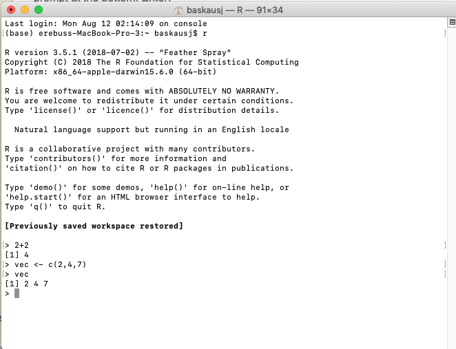
In the console you can type commands and the result may be shown below what you have typed. For example, entering
2+2
will immediately display the answer to that mathematical calculation.
The second command that was entered:
vec <- c(2,4,7)
assigns three numbers to an R data structure called a vector. In this case the vector is given the name vec. Assinging the numbers to the vector vec does not produce any visible result on the console. Instead, the vector is stored in a part of the computer’s memory called the workspace. To display the contents of vec, enter its name in the console.
Data stored in the workspace will persist during the session. When the session is closed using the q() command, the workspace can be saved to the hard drive and will be reloaded the next time R is restarted.
The RStudio GUI
RStudio is a typical integrated development environment (IDE) in that it provides additional tools to make the process of developing scripts easier. It has a graphical user interface (GUI) that displays things without necessarily having to enter lines of commands.
When RStudio is launched, it looks something like this:
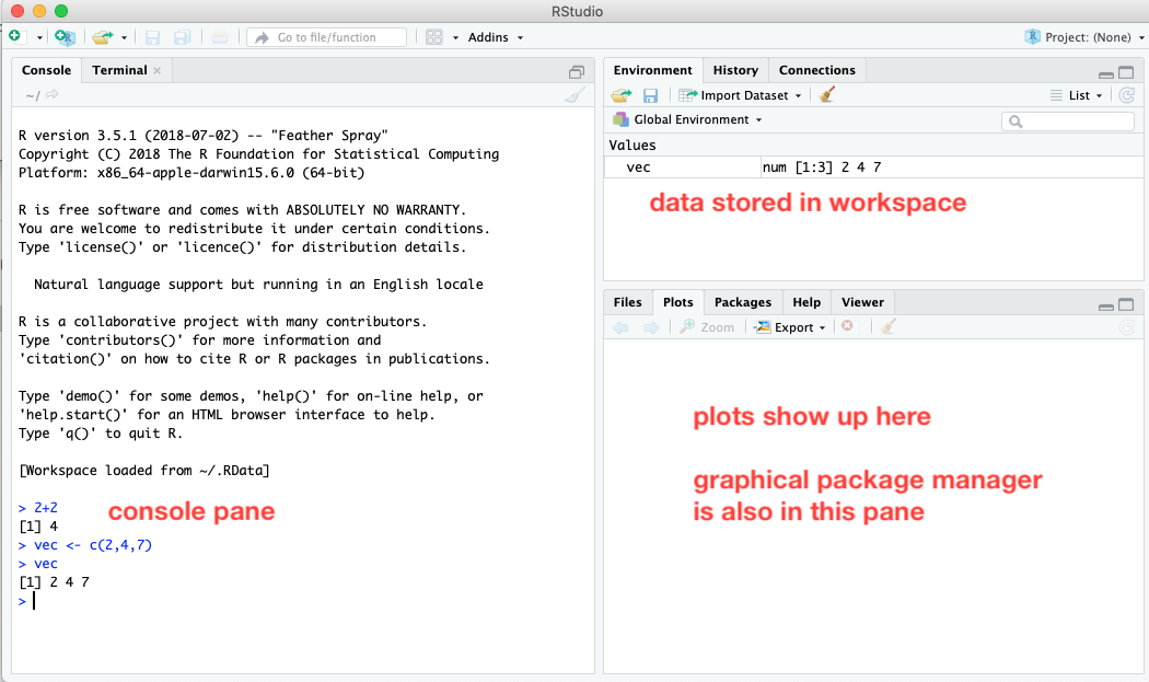
The GUI is divided into several panes. On the left there is a pane with two tabs - by default the Console tab is selected. The console pane behaves exactly like the console as if it were launched in a Terminal or Command Prompt window. As shown in screenshot above, the same commands as before were typed into the console pane, with the same results. However, in the upper right pane, under the Environment tab, any data structures stored in the workspace are listed. We can see that the vector vec shows up, along with a summary of its contents. To clear the workspace, you can click on the little broom icon.
There is a third pane in the lower right that serves additional purposes. Its Plots tab will show the results of any graphs that are generated. Its Packages tab provides a graphical interface for installing and loading packages (an alternative to loading them via text commands in the console).
Opening an editor pane
Typing commands directly in the Console pane is a fine way to experiment and carry out simple tasks. However, it’s not the best way to develop more complex multiline scripts. RStudio has a built-in editor that can be used to build scripts. To begin a new script, select New File from the File menu, then R Script. A fourth pane will appear in the RStudio window, in a tab that defaults to Untitled1.
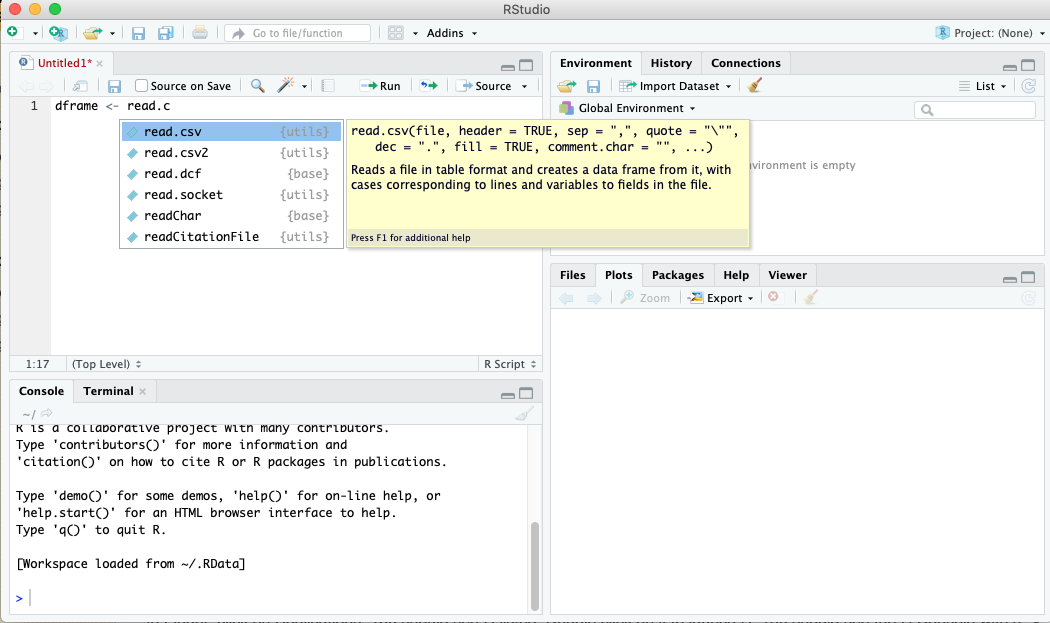
As you work in the editor pane, suggestions will pop up as you type, as shown in the screenshot above. The following is an example of a two-line script that runs a t-test of means on a simple dataset.
heightsDframe = read.csv(file="https://raw.githubusercontent.com/HeardLibrary/digital-scholarship/master/data/r/t-test.csv")
t.test(height ~ grouping, data=heightsDframe,
       var.equal=TRUE,
       conf.level=0.95)
Notice that although the script takes up four lines, the last three are considered a single line of code, since the t.test function doesn’t come to an end until the final closing parenthesis is reached. Here’s what the code looks like when pasted into the RStudio editor pane:
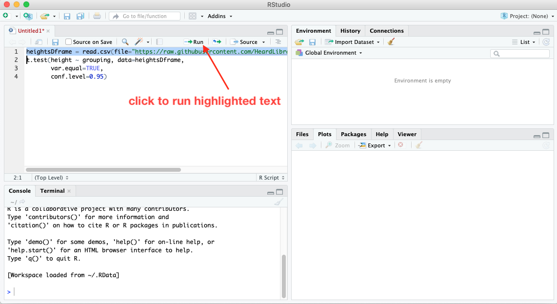
You can run code that’s in the editor pane one line at a time, or all at once. To run a single line of code, highlight it (or simply place the cursor somewhere on the line). Then click the Run button at the top of the pane.
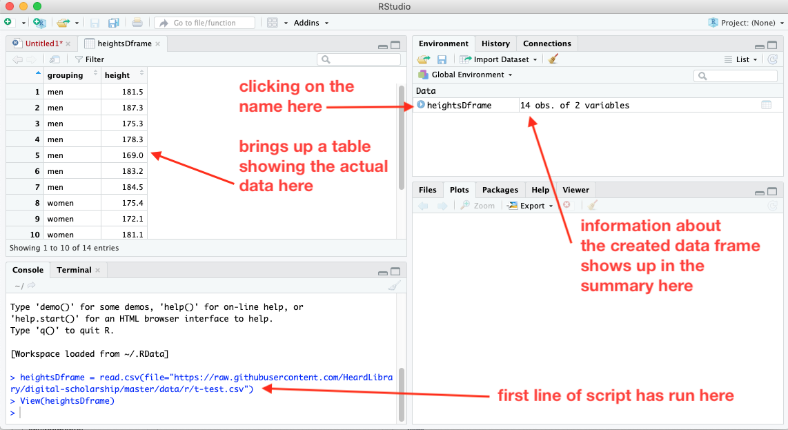
The first line creates a data structure called a data frame. After clicking on the run button, we see in the console pane that the first line has run, and a summary of the data frame has appeared in the workspace. The data are too extensive to display in the workspace summary, but if you click on the name of the dataframe in the summary, the View function will run in the console, and a new tab will open up in the upper left pane showing the structure of the data in the data frame. To return to the scipt, click on the Untitled1 tab.
To run the rest of the script, highlight the second line (or put the cursor on the second line), and click run again.
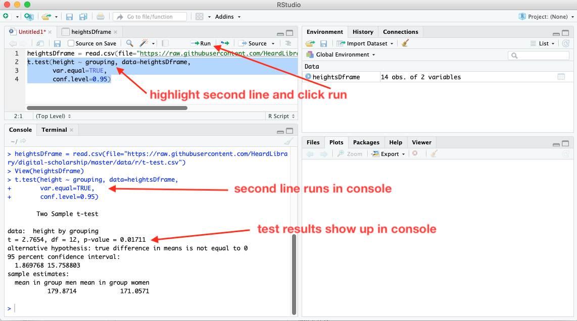
The command in the second line of the script appears in the console window, along with the results of the test.
If you want to run the entire script at once, just highlight the entire script in the editor window and click run. Each line will be run one at a time in the console window.
Loading packages
Because there are so many ways to use R, it is not practical to include all of the necessary code as part of the basic R application. Instead, additional capabilities are added to R by loading packages that add functionality to the basic application.
The particular package that you need to complete some task may or may not already reside on your local computer. If you have installed the Anaconda management system, most of the packages that you are likely to ever need will have already been downloaded and installed on your computer. Otherwise, if you are missing a necessary package, you will need to download it from a Comprehensive R Archive Network (CRAN) site. This can be done using a text command in the console. However, if you are using RStudio, you can use its graphical interface to manage the download.
In the following example, we will need to use two packages: Hmisc and ggplot2. To determine whether your computer already has ggplot and Hmisc installed, click on the Packages tab in the lower right pane.
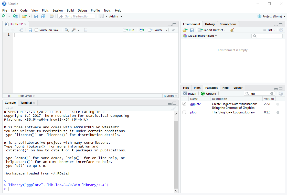
In the search box, start typing ggplot2. As you type, packages with matching names will be screened. If you see ggplot2, click the checkbox to the left of its name. When you check the box, RStudio will run the library function for you in the console pane, and load the package. If ggplot2 does NOT show up in the list, then ggplot2 isn’t yet installed on your computer. Click the Install button. If prompted to create a personal library, click Yes.
An Install Packages window will pop up. You can leave the Install from: option at its default “Repository (CRAN..”. In the Packages box, type
ggplot2
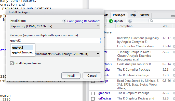
A bunch of lines will scroll up the console window. When it says “The downloaded binary packages are in…” you’re done. The package should now appear in the list of packages in the Packages pane in the lower right, where you can check its box.
Repeat the process for the Hmisc package.
Creating a plot
We will now create a bar chart with error bars using the same data that we used in the t-test.
R has a number of relatively simple, built-in plotting functions that do not require installing any additional packages. However, the ggplot2 system is very popular and widely used because it allows the user to control many features of the plot. The down side of this level of control is that it tends to make the plotting function complicated. If you are interested in data visualization using R, we highly recommend the book R for Data Science, which is available online for free (and has an awesome picture of a kākāpō on its cover!). This book introduces the “grammar of graphics” philosophy that underpins the ggplot2 package.
If you have worked through the examples so far, the data that we want to plot is already loaded into the workspace as a data frame called heightsDframe and you only need to issue the command to generate the graph. If you have skipped down to this point, you will first need to load the data into the data frame using this command:
heightsDframe = read.csv(file="https://raw.githubusercontent.com/HeardLibrary/digital-scholarship/master/data/r/t-test.csv")
If the data frame is loaded into the workspace, you should see it listed in the Environment pane in the upper right.
The command to create the plot can be given by entering this function in the console:
ggplot(data=heightsDframe, aes(x=grouping, y=height, fill=grouping))+ stat_summary(fun.y = mean, geom = "bar") + stat_summary(fun.data = mean_cl_normal, geom = "errorbar", width = 0.3)
After the ggplot function executes, the resulting bar graph will appear in the Plots tab of the lower right pane.
Here’s an explanation of how the features of the plot are controlled. Replace the appropriate value for the square brackets and the text within.
ggplot(data=[name of dataset], aes(x=[name of column to use for grouping bars], y=[name of column to use for y-axis value], fill=[name of column to use for determining bar color]))+ stat_summary(fun.y = mean, geom = "bar") + stat_summary(fun.data = [value to be used for error bars], geom = "errorbar", width = 0.3)
The example shows uses “mean_cl_normal” to produce error bars for 95% confidence intervals. Use “mean_sdl” for standard deviation error bars or “mean_se” for standard error of the mean error bars.
There are other options that can be used to change the width of the bars, whether the bars are outlined in black, etc. You can experiment with it and Google to find out more about how to embellish the plot.
You can also set the values of the axis labels to be something other than the defaults taken from the column headers by adding a labs() function to the command, as in this example:
ggplot(data=heightsDframe, aes(x=grouping, y=height, fill=grouping))+ stat_summary(fun.y = mean, geom = "bar") + stat_summary(fun.data = mean_cl_normal, geom = "errorbar", width = 0.3) + labs(x = "gender", y = "height (cm)")
You can use the Export function (found immediately above the plot) to copy or save the plot. If you chose the Save Plot as Image option, you can save the plot in a variety of image formats and also mess with the plot resolution.
Scripting the plot
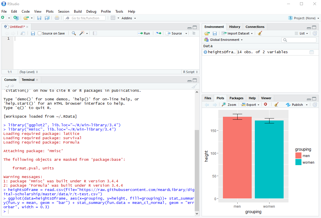
The entire process of loading the packages, loading the data into the data frame, and generating the plot can be included in this four line script:
library("ggplot2")
library("Hmisc")
heightsDframe = read.csv(file="https://raw.githubusercontent.com/HeardLibrary/digital-scholarship/master/data/r/t-test.csv")
ggplot(data=heightsDframe, aes(x=grouping, y=height, fill=grouping))+ stat_summary(fun.y = mean, geom = "bar") + stat_summary(fun.data = mean_cl_normal, geom = "errorbar", width = 0.3) + labs(x = "gender", y = "height (cm)")
Here’s the result:

If you paste the script into the editor window, you can run the whole thing at once by highlighting all four lines, then clicking Run. You can also save the file by clicking on the save icon above the editor text, or selecting Save from the File menu. (The default for R scripts is to use the file extension .R, e.g. demo-graph.R.) If you save the script, you can load it again later to use as a template for future modifications of the script. In the screenshot above, the script has been saved, so you see “demo-graph.R” as the name in the tab instead of “Untitled1”.
Continue to Introduction to R data structures
Revised 2019-08-14

Questions? Contact us
License: CC BY 4.0.
Credit: "Vanderbilt Libraries Digital Lab - www.library.vanderbilt.edu"