return to Where do I go from here?
go to Getting started with R and RStudio
R Scripts for Basic Stats
This page contains scripts for several basic statistical tests and one more complex test (ANOVA). This lesson assumes that you have RStudio installed on your computer and are familiar with the lessons Navigating around in RStudio and Introduction to R data structures. If you haven’t already studied them, you should look at them first.
In each test, the first line of the script as written retrieves a CSV file from the DiSC Office’s GitHub code repo using a URL. If you are going to use the script with your own data from your hard drive, you will need to substitute the following line for the first line of the script:
myDataFrame <- read.csv(file.choose())
You’ll need to replace myDataFrame with whatever name was used for the data frame in the example. See Methods for reading CSV data into data frames for more information.
t-test of means
A t-test of means assesses the difference between two levels of a single factor. In this example, the factor is sex and the levels are men and women. The dependent variable (response) is named height and has numeric values. In order for R to carry out the test, the data need to be arranged with one column for the grouping variable designating sex and a second column containing the height data, like this:
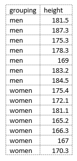
Data arranged in this manner is called “tidy data”. Important note: because of the difference between the way that R handles numeric and string data when it loads it into a data frame, it is important that the levels in any grouping variable that you use in the source CSV file contain non-numeric characters. See Data types in data frames and tibbles for details.
Here’s the script to perform the t-test of means on these data:
heightsDframe <- read.csv(file="https://raw.githubusercontent.com/HeardLibrary/digital-scholarship/master/data/r/t-test.csv")
t.test(height ~ grouping, data=heightsDframe, var.equal=TRUE, conf.level=0.95)
You can run the script by pasting it into the editor pane, highlighting (selecting) both lines, and clicking the Run button. You could also enter each of the two lines one at a time in the Console pane, but that would be more work. If you have forgotten how the RStudio GUI is laid out, please review The RStudio GUI.
The results of the test show up in the Console pane. The P-value of 0.01711 indicates that the heights of men and women are significantly different based on these data.
In height ~ grouping of the second line of the script, height is the name of the column containing the data (dependent variable) and grouping is the name of the column containing the grouping variable (independent variable). We can see that the columns in the data frame are laid out in this way by clicking on the name of the data frame (heightsDframe) in the workspace summary in the upper right pane of RStudio. The data frame will be displayed in table form in the upper left pane where you can verify that height and grouping are actually the names used in the headers of the appropriate columns. If the data you want to analyze have different column headers, you’ll need to change the script to the appropriate column names.
paired t-test
A paired t-test differs from a t-test of means in that each particular observation in one of the two groups is paired in some way with a particular observation in the other group.
In R, the pairing of observations is done by placing the observations of the two groups in two vectors. Because the items in the vectors are ordered, R knows to associate the first item in the first vector with the first item in the second vector, etc. The general form of the function for paired t-test is:
t.test(firstVector, secondVector, paired=TRUE)
If we want to read in the values from a CSV file, we’ll want to lay out the file differently from the way we laid out the data in the file for the t-test of means:
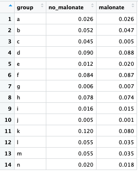
The data for each group are located in a separate column since we will want to be able to refer to the group data by column name. Recall from the lesson on data structures that a data frame is essentially a list of vectors, with each vector serving as a column. So for the first and second vector we input into the t-test() function, we can insert a column from the table.
This example file has a third column (“group”) with a letter identifying each pair, but it isn’t necessary for the test and R will simply ignore it. Here’s how we can perform the test on these data comparing enzyme reaction rates in the presence and absence of malonate:
malonateDframe <- read.csv(file="https://raw.githubusercontent.com/HeardLibrary/digital-scholarship/master/data/r/paired-t.csv")
t.test(malonateDframe$no_malonate, malonateDframe$malonate, paired=TRUE)
Notice that in this example, we referred to the data in a particular column using the $ notation (e.g. malonateDframe$no_malonate for the data in the “no_malonate” column). R treats the column data from the data frame as it would a vector when it inputs it into the t.test function.
chi-squared goodness of fit test
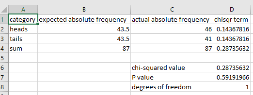
When running a chi-squared goodness of fit test using R, the actual frequencies (i.e. the observed frequencies) must be absolute (i.e. counts). The expected frequencies must be relative (i.e. the probabilities or proportions expressed as decimal fractions). This differs from the way the test is conducted in Excel where both the actual and expected frequencies must be absolute. For example, an Excel example to calculate whether coin flips differ from the expected equal probability of heads and tails looks like this:
while the setup in R would look like this:
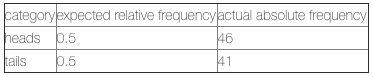
To carry out the test, we need two vectors: one containing the observed values as counts and another containing the expected values as relative frequencies. For the example above, here’s how we would do the test:
actualAbsFreq <- c(46, 41)        # actual absolute frequency: (heads, tails)
expectedRelFreq <- c(0.5, 0.5)      # expected relative frequency: (heads, tails)
chisq.test(x = actualAbsFreq, p = expectedRelFreq)
Note that the order of the items in the observed vector need to correspond to the order in the expected vector.
chi-squared contingency test
Here is a contingency table for data to test whether the sex of the second child in families is independent of the sex of the first child.
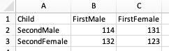
In R, the data for a contingency test must be in the form of a data structure called a matrix. Details of the matrix data structure are beyond the scope of this lesson - we will simply convert the data from a data frame into a matrix using a function. Here is the script:
childrenDframe <- read.csv(file="https://raw.githubusercontent.com/HeardLibrary/digital-scholarship/master/data/r/contingency.csv")
childrenMatrix <- as.matrix(childrenDframe[,-1]) # convert data frame to matrix, removing first column
chisq.test(childrenMatrix, correct=FALSE)      # don't do Yates' correction
The first column of the table is to help us keep the combinations straight, but is not needed by R. So when we convert the data frame into a matrix in the second line of the script, the ,-1 removes the first column before the conversion.
In the third line of the script, correct=FALSE turns off Yates’ correction, which can be used when contingency tests have expected cell frequencies of less than 10.
Regression
Using these fake data, we want to test whether there is a significant effect of treat size on the rate at which dogs wag their tail.
To perform a regression using R, we usd the linear model function lm(). The first argument of the function contains the dependent variable (wag_rate), followed by a tildle and the independent variable (treat_size). After running the model, we ask R to summarize the results:
dogtailDframe <- read.csv(file="https://raw.githubusercontent.com/HeardLibrary/digital-scholarship/master/data/r/dog-tail.csv")
model <- lm(wag_rate ~ treat_size, data=dogtailDframe)
summary(model)
The results table looks like this:
Call:
lm(formula = wag_rate ~ treat_size, data = dogtailDframe)

Residuals:
      1       2       3       4       5
-0.1834 -1.3108  1.3948  1.3911 -1.2917

Coefficients:
            Estimate Std. Error t value Pr(>|t|)
(Intercept)  -1.2045     1.3716  -0.878  0.44451
treat_size    1.4522     0.2416   6.011  0.00923 **
---
Signif. codes:  0 ‘***’ 0.001 ‘**’ 0.01 ‘*’ 0.05 ‘.’ 0.1 ‘ ’ 1

Residual standard error: 1.56 on 3 degrees of freedom
Multiple R-squared:  0.9233,	Adjusted R-squared:  0.8978
F-statistic: 36.13 on 1 and 3 DF,  p-value: 0.009225
We can get the slope and intercept from the Coefficients section: the slope is in the Estimate column for treat_size (1.4522). The intercept is in the Estimate column for (Intercept) (-1.2045). The last lines of the results provide the other two things we are likely to be interested in: the R-squared value and p-value.
ANOVA
The setup of a data table to carry out an ANOVA in R uses grouping variables in the same manner as the t-test of means. Please review the description of grouping variables and the warning about numeric values in grouping variables in the section about running a t-test of means.
Some advice: When setting up tables with grouping variables, it’s best to type the value of each factor only once and use copy and paste to fill in all of the other cells. This helps you avoid problems with the test caused by typographical errors.
Single factor ANOVA
The following example uses data from an electroretinogram to test whether there are differences in a cockroach eye’s sensitivity to red and green light.
ergDframe <- read.csv(file="https://raw.githubusercontent.com/HeardLibrary/digital-scholarship/master/data/r/red-green-anova-example.csv")
model <- lm(response ~ color, data = ergDframe)  # fit a linear model to the data
anova(model)  #run the ANOVA on the model
As was the case with the t-test of means, in the lm() function, the name of the data column is the first argument of the function, followed by a tilde and the name of the grouping variable.
Since the format required for a single factor ANOVA with two categories is exactly the same as the format required for a t-test of means, the same file could be used for either test. Since a single factor ANOVA with two levels is statistically equivalent to a t-test of means, the resulting P-values should come out the same.
Unlike a t-test, which can only compare two groups, a single factor ANOVA can check for differences among three or more levels of a treatment. For example, if you replace the following line for the first line in the script, the ANOVA will compare the effect of red, green, and blue light based on these data:
ergDframe <- read.csv(file="https://raw.githubusercontent.com/HeardLibrary/digital-scholarship/master/data/r/color-anova-example.csv")
Two factor ANOVA
The setup for a multi-factor ANOVA in R is similar to a single factor ANOVA except that there are two columns for grouping variables instead of one. In this example (using fake data), we are simultaneously examining the effect of soap and triclosan (an antimicrobial agent) on the bacteria found on hands after washing:
soapDframe <- read.csv(file="https://raw.githubusercontent.com/HeardLibrary/digital-scholarship/master/data/r/fake-soap-experiment.csv")
model <- lm(counts ~ soap + triclosan, data = soapDframe)
anova(model)
Notice that the format of the lm() function that fits the linear model is very similar to the single-factor ANOVA. The only difference is that there are two grouping variables (“soap + triclosan”) specified after the tilde, instead of one. Here’s the ANOVA table from the output:
Analysis of Variance Table

Response: counts
          Df   Sum Sq Mean Sq F value Pr(>F)
soap       1  4704500 4704500  7.0898 0.0164 *
triclosan  1   264500  264500  0.3986 0.5362
Residuals 17 11280500  663559
---
Signif. codes:  0 ‘***’ 0.001 ‘**’ 0.01 ‘*’ 0.05 ‘.’ 0.1 ‘ ’ 1
Since this is a two factor ANOVA, there is a line in the ANOVA table for each of the two factors, and each factor has its own P-value. The star after the soap P-value indicates that the factor is significant at the P < 0.05 significance level as shown by the key of significance codes below the table. If the P-value had been less than 0.01, two stars would have been used, etc.
ANOVA with blocking
We can run an ANOVA test in the same way when one of the two factors is a block effect. (Note: we are oversimplifying in this example, since when one of the effects is random we should be making modifications to the script. But that’s beyond the scope of this lesson.) Here is the script to analyze the cockroach color data from before, but this time including the individual roach as a block:
ergDframe <- read.csv(file="https://raw.githubusercontent.com/HeardLibrary/digital-scholarship/master/data/r/color-anova-example.csv")
model <- lm(response ~ block + color, data = ergDframe)
anova(model)
return to Where do I go from here?
go to Getting started with R and RStudio
Revised 2019-08-19

Questions? Contact us
License: CC BY 4.0.
Credit: "Vanderbilt Libraries Digital Lab - www.library.vanderbilt.edu"